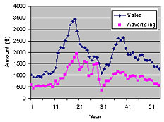
As a result of a lawsuit in the early 20th century, 54 years worth of annual sales and advertising data for the Lydia Pinkham company became public knowledge. Lydia Pinkham sold a patent medicine for "women's problems." These data are often used in textbooks to illustrate modeling techniques, as we will do here.

The following graph shows the data graphically. Although it would seem feasible to divide the data into two halves in order to do cross-validation, we will keep a single dataset for illustration purposes.

To start with, we will model the data as a simple linear correlation between the sales in a year (S_i) and the advertising budget in the same year (A_i).

The resulting model is:

S_i = 488.83 + 1.4346× A_i

R² = 0.711 F = 64.

This model would seem to indicate a strong return on the advertising dollar. It explains about 71% of the variance in the data, as indicated by the R² value. However, when we start looking at more complicated models, the picture changes.

Next, we will model the data using a linear time-series model, also called an autoregressive (AR) model, which is a form of Box-Jenkins model. We will initially test for models using only the previous year's sales (S_i-1) and advertising budget (A_i-1) to predict the current year sales (S_i). Thus our set of candidate lags is {0,1}. The zero lag is used only for advertising. In other words, sales in a particular year was modeled as a function of the same year's advertising budget, and both sales and advertising in previous years. To keep the model linear initially, we will set multiplicands = {1} and exponents = {1} in the TaylorFit software as well. We used TaylorFit in a manual mode.

The resulting model is:

[Linear AR(1) Model] R² = 0.915 F = 130.

S_i = 154.07 + 0.58944×Ai + 0.95546×S_i-1 - 0.66006×A_i-1

This seems to indicate that the company got almost all of last year's sales back, and that advertising produces a 58% return, which unfortunately is completely canceled out by the previous year's advertising.

This is a different story from that described by the simpler model. This shows how a model could mislead by not including all relevant effects. This problem could occur by not including nonlinearities, as well.

Next, we incremented the set of lags until we could not improve the model with additional lags.

[Linear AR(2) Model] R² = 0.921 F = 110.

S_i = 202.48 + 0.51683× A_i + 1.2111× S_i-1 + 0.51716× A_i-1 - 0.31703× S_i-2

Only a single additional term appears: sales from two years previous. Furthermore, it is a negative term. The presence of both positive and negative terms for both sales and advertising indicates the presence of an oscillatory behavior. This is the best linear model that we found.

The third step was to allow the simplest kind of interaction in which terms consisting of cross-multiplied independent variables were included as candidate terms for the model. In TaylorFit this is accomplished by changing the set of multiplicands to {1,2}. The resulting model is:

[Simple Interaction Model] R² = 0.928 F = 150.

S_i = 0.96474× A_i + 0.97122× Si-1 - 0.517647× A_i-1 - 1.5621×10-4 × S_i-3×A_i

It is interesting that the intercept term disappears, and the term for sales from two years ago is replaced by an interaction between sales from three years previous and advertising in the previous year. This may indicate a negative effect of advertising on long-time customers. This term is very significant (the t-statistic is 4.25).

Finally, we began exploring exponents other than {1}. Specifically, we tried exponents = {1, -1} and exponents = {1, -1, 2}, in order to introduce ratios and curvature into the model. The result was:

[Complete PARX Model] R² = 0.960 F = 150.

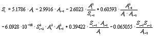
The smallest (absolute) t-statistic for the terms in this model is 2.29, for the last term. The next smallest is 4.56. So, the terms are very statistically significant. You can also see that the error (computed as 1-R²) is about half that of the best linear model. In spite of the increased complexity, this model also has a higher F-statistic than the linear model. This is confirmation that the complexity is warranted, since the F-statistic is more conservative than other criteria such as the R² or MSE, in that it contains a greater penalty for model complexity.

However, because of the model's complexity, it will be difficult to interpret individual terms in any deterministic way, as was done for the last term in the simple interaction model above. What should be done in this case is to analyze the model graphically, by computing sensitivities, and by testing the model for a variety of cases of interest. The model can be used to simulate various strategies for setting an advertising budget, for example.

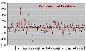
To demonstrate one way to evaluate the model, the graph below compares the residuals (errors) for three of the models: the linear AR(2) model, the simple interaction model, and the complete PARX model. You can see that the largest residuals are produced by, in most cases, the linear model and the simple interaction model.