A company had 54 retail stores that sold industrial supplies and equipment. They wanted to understand what factors controlled the stores' profitability. They had measured thirteen variables that they thought could have an affect on the gross margin (GM). The thirteen variables were:

• SE - The ratio of sales of supplies to sales of equipment
• M - Market share in the local area
• Y - Years the store was at that location
• S - Total sales
• W Ratio of Walk-in sales to delivered sales
• Q - Store Quality (a qualitatively judged value from 1 to 3)
• C - Intensity of local competition
• I - Industrial concentration in local area
• RU - Rural vs. urban location
• V - Highway visibility
• N - # of staff
• YS - Average years of service of staff
• NS - # of salespersons

Note that when the data have been collected for each store, they can be contained in a table or spreadsheet with 54 rows and 14 columns - one column for gross margin, and thirteen for the independent variables.

The question of interest is: Which variables significantly affect gross margin, and how do they affect it? A standard approach to this question for this kind of data is to use multilinear regression. By using the stepwise regression procedure on these data, we obtained the following model:

GM = 0.46·SE + 0.13·M R² = 0.62

The modeling process was then continued using TaylorFit. Candidate terms with a maximum of two multiplicands were considered, and the list of possible exponents (other than zero) was {1, -1}.

The use of the negative exponent allowed TaylorFit to explore the possibility that ratios of independent variables might contribute significantly to the fit. The best model that resulted was:

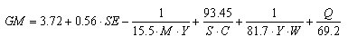
;R² = 0.82

The relative amount of error not accounted for by the model is 1 - R². For the MLR model this is 0.38. For the MPR model it is 0.18. That is, the additional terms reduced the error by more than half. More importantly, the MPR model reveals some important information.

First of all, note that the SE term is still there, but with a larger coefficient. This shows the bias of the linear model. By ignoring the effect of other variables, the sensitivity of GM to SE was underestimated.

Secondly, in the MPR model the GM still increases with M, but it's a negative inverse effect, indicating a saturation behavior (increasing, but leveling off).

Furthermore, the effect of M depends upon Y. That is, M and Y interact. Linear models are incapable of describing either the curvilinear behavior or the interaction shown in this term. These behaviors can be seen more clearly in the following figure:

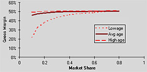
This figure shows the saturation effect of market share on gross margin. However, it is interesting to note how Y affects this behavior. Basically, the saturation effect is very pronounced at low Y (relatively new stores), but for average or older stores, the curve is flat, indicating that market share has little effect on gross margin for such stores. This is the kind of behavior that cannot be described with linear models.

(Incidentally, this model can be interpreted various ways. It might indicate that stores with low market share need only to become more established before they are profitable. Alternatively, it might be found that such stores disappear from the database, that is, they go out of business, before they reach older status. The investigator should examine the data carefully before drawing conclusions.)

Another point that the model makes is that six of the independent variables had no measurable effect on gross margin. This kind of information is also potentially useful to the company.