Chaotic time-series are a particularly challenging class of nonlinear processes. Chaos, in the mathematical sense, has been defined as "extreme sensitivity to initial conditions."

In a non-chaotic process, if you do two simulations using two different starting points (represented by points in the "phase plane") that are close together, the distance between the two points will decay to zero, stay constant, or increase linearly. In a chaotic process the distance increases exponentially. Eventually, the trajectory of the two points will appear unrelated (i.e., uncorrelated). For example, if you tossed a pair of oranges into a stream, they would flow together if the stream flow were slow and smooth. But if it were turbulent, the motion of the two oranges would quickly become unrelated.
The coefficient of exponential increase in distance between the points is called the Lyapunov coefficient (°). If ° is negative or zero for a process, then it is non-chaotic. If ° is positive, then the process is chaotic.

Chaotic time-series data often look random but aren't. Researchers studying a process may be interested in determining if "noisy" behavior is really randomness, or actually deterministic chaos. This makes a big difference in our ability to make predictions, because true noise is inherently unpredictable, whereas chaotic processes can be very predictable (in the short term). Economic time-series are an example of one type of data that people are interested in distinguishing chaotic from random behavior.
A technique that proves capable of (a) determining if a process is chaotic, and (b) developing a predictive model of the processes may find wide applicability.

A Test Case: The Lorenz Equations

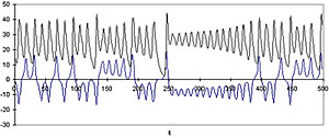
The Lorenz equations are a set of three differential equations based on a model of heat-driven fluid flow (thermal convection). The three equations predict the changes in three variables, denoted by x, y, and z, over time. The figure below shows an example plot of how x, and z vary with time (y behaves similarly to x, the lower curve).

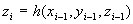
If you plot any two of the variables versus each other, you get a phase plane plot. Here is an example of a plot of y versus x:

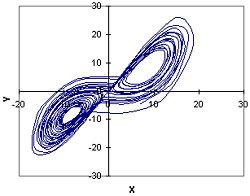
This plot shows the complex phase plane trajectory that never loops back on itself, explodes to infinity, or converges to a fixed point, as non-chaotic processes will do. The "butterfly-shaped" region containing the chaotic trajectories in the phase plane is called an attractor.

Using MPR to Identify Chaos

The MPR model was found to be able to identify the nonlinear dynamic behavior of the Lorenz equations, as reflected in the geometry of the attractor and by calculation of its Lyapunov exponents. The technique was applied to times series data obtained from simulations of the Lorenz equations with and without measurement noise.

The Lorenz equations were used to generate a time-series of values of x, y, and z. Then, an MPR model was developed to predict each variable, using only lag-1 values of x, y, and z. That is, three MPR models were generated:

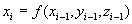
For example, a portion of the equation for x is (the subscript i-1 is dropped on the right side for simplicity):

x_i = x + 3.4070×10^-7×xz⁵ + 4.7659×10^-1×y - 3.4949×10^-3×xz² - 1.5647 ×10^-4×x³ + . . .

Then, using these models alone (without reference to the original data or the original Lorenz equations), a new sequence of values of x, y, and z were generated. When x was plotted versus y, the following trajectory was obtained:

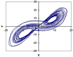
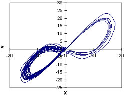
You can see that it has the same appearance of the phase-plane trajectory of the Lorenz equations. Even if random noise was added to the data before modeling (at a level of approximately 10% of the variance of the data), an approximation to the Lorenz attractor could still be recovered from the data, although additional lags (lag 1, 2, and 3) had to be used. The resulting attractor still has the butterfly geometry:

A final test was to compute the Lyapunov coefficients of the MPR models and compare them to the known values of the Lorenz equations. Three values could be computed for this system. The values for the MPR models were computed using a standard procedure (Wolf, 1986). The results are:

Lorenz equations	1.30	-0.002	-20.7
MPR, no noise	1.33	-0.065	-21.3
MPR, with noise	1.09	-0.46	-18.0

This shows that the MPR models accurately reproduced the Lyapunov coefficients in the case of the model fitted to the noise-free data. In the case of the noisy data, the first and third coefficients were predicted with reasonable accuracy, although the second is inaccurate. However, it is the first coefficient, the positive one, which shows the chaotic nature of the process, and dominates the behavior of the system.

The MPR models were developed from the data, and not using the Lorenz equations themselves. And yet they could be used to reproduce both the phase plane trajectory and the Lyapunov coefficients of the original equations. This illustrates the power of MPR to discover relationships underlying the data, including the dynamic behavior of the process, and to distinguish noise from chaos.

In turn, this demonstrates the capability of MPR to model some of the most challenging types of processes.