We will consider applications to data formed from measurements sampled at equal time intervals, TAU, of n_x input, state and output variables. Here we will not distinguish among these types of variables. The data point x[i,j] is the measurement of variable i taken at time step j. In general, each variable may depend upon previous measurements of itself and the other variables, except for input variables which do not depend upon state and output variables.

A type of ARMA model applied to such systems is the vector autoregressive (VAR) model, in which a prediction is found by a linear combination of previous (lagged) measurements, x[i,j-l]:

[1]

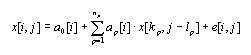
where 1 ³ i ³ nx, 1 ³ kp ³ nx; kp ¹ i if lp = 0; lm+1 ³ j ³ nd; lm ³ 1 is the maximum lag; and e[i,j] is the error in the model prediction. The parameters a are determined by fitting the model to a set of data. An identification process is used to select which of the possible terms in equation 1 contribute significantly to the model, and only those terms are retained.

More complex behaviors, such as coupled sensitivities between variables or curvature in the responses, could be included in an VAR model by adding polynomial terms to equation 2:
[4a]

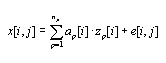
[4b]

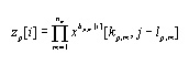
The additional parameters of this model compared to equation 1 are bp,m, the (usually positive integer) exponents for each multiplicand in each term, and nm is the maximum number of multiplicands in each term of the model. The indices i, j, k, and l are defined as for equation 1.

The model is made tractable by restricting the values that can be taken on by the exponents, b, the lags, and the value of nm, and by including in the model only those terms which contribute significantly to the fit. The fitting procedure involves a stepwise selection process, described below, in which a set of candidate terms are tested for inclusion in the model.

The restricted set of candidate terms are formed as follows: First, a list of n_e candidate exponents is selected, not including zero which is always assumed. Then, a list of lags to be considered is formed. Formation of this list may be an iterative process involving sequentially adding lags until the model cannot be improved. In some cases discontinuous lags may be added to the list to represent expected seasonal effects. If lag 0 is included in the list, then variable i is being correlated to "current" values of the other variables, and variable i, lag 0 must be excluded from the candidate terms. The total number of lags in the list, which may include lag zero, is n_l.

The stepwise procedure then selects a set of polynomial terms from the candidates that optimizes the fitting criteria. The resulting MPR model can thus be completely specified by a table containing the following information for each term:

kp,1, lp,1, b1; kp,2, lp,2, b2; . . . kp,nm, lp,nm, bnm; ap

The Number of Candidate Terms
Adding lagged values increases the number of "independent variables." The total number of independent variables, n_v will be:
[6]

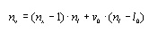
where l₀ equals one if the list of lags includes zero, and equals zero otherwise, and v₀ equals one if lagged dependent variables are included as independent variables, and zero otherwise.
The maximum value that nm can take is n_v. If n_m = n_v, then the total number of candidate terms is:
[5]

This may result in a large number of terms to be tested for selection into the model. For example, if there are three independent variables (n_x=4) and no lags (n_l=1), and ten exponents (n_e=10), then there are n_t = 1331 possible terms. Experience with a wide variety of datasets has shown that n_m can often be restricted to two or three. For n_m £ n_v:
[7]

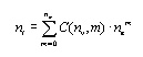
where C(n_{v, m}) is the number of combinations of n_v objects taken m at a time. For the example above, if n_m = 2, the number of candidate terms drops to 331.