To understand what MPR does, we will first look at some basics of empirical modeling.

A model is something that mimics the behavior of some real system of interest. Our interest here will be in mathematical models, which are usually equations, and which predict some result based on factors that influence that result.

Mathematical models can be mechanistic or empirical. A mechanistic model is one that is derived from more fundamental principles. For example, we could use the laws of physics to derive a mechanistic model that predicts the motion of a building in an earthquake.

In many cases, a system is too complicated to predict from fundamental principles. Almost anything to do with human behavior, such as economic systems, will fall into this category. But many physical systems can also be beyond mechanistic modeling. Some aspects of weather prediction would be an example. In such cases, we use empirical modeling. Literally, this means modeling based on experience. In practice, an empirical mathematical model is an equation whose coefficients are adjusted to match a given set of data.

Simple Linear Regression

One of the simplest examples and most familiar forms of empirical model is the fitting of a straight line through some data. The equation of a line is:

Y = a₀ + a₁ · X

For example, if we measured the flow of water in a stream and the amount of rainfall in its catchment area over a period of time, we might find that the stream flow was equal to a minimum dry weather value, plus some amount that was proportional to how much rain fell in the last 24 hours: Flow = a₀ + a₁ · (Rainfall) In this case, the intercept a₀ is the dry weather river flow (the flow when Rainfall = 0), and the slope a₁ is the constant of proportionality.

Simple linear regression is a mathematical technique that determines the values of a₀ and a₁, give a set of data showing the river flow and rainfall for a number of days. This determination is called fitting the model. When we fit a straight line to the data by linear regression, we are assuming that the data can be well-described by a line. Regression will give us the equation of a line whether or not that is the best equation to use. The best way to see if the fit is a good one is to look at a graph of the data and the fitted line.

In models of this sort one variable will be the result or outcome, and is called the dependent variable. There will be one or more causative variables, called independent variables. In the example above, rainfall is the independent variable, and river flow is the dependent variable.

Systems and Models
Consider some outcome that has several causes, or inputs. For example, if the outcome is the number of tons of corn produced by an acre of land, the causes could be the amount of nitrogen fertilizer added, the amount of phosphorus fertilizer, and the amount of irrigation water supplied.

Or, if the outcome is the Dow Jones stock market index, the inputs might be the Fed interest rate, the unemployment rate, and the money supply (if only it were so simple!).

Of course, one might want to add other inputs. Selecting the input variables depends upon the system of interest, and is part of the art of modeling.

To make things clear, let's just consider two or three inputs, which we'll call Q, R, and S, and we'll call the output Y. The red box is the system: the real thing whose behavior we are trying to predict.

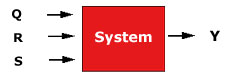
We're looking for a rule, which we call the model, such that if we gave it values for the input variables, it would predict what the output Y would be. Ideally, the model should behave the same as the system. In practice, of course, no model is perfect. For example, crop productivity will also depend upon temperature, amount of sunlight, and many other factors. But we can limit ourselves to a fewer number if those other factors are held at constant levels, or if they are significantly less important determinants of the outcome.

Multilinear Regression (MLR)

When there is more than one independent variable, the simplest model is called multilinear regression (MLR). For example, if Y depended on Q and R, a MLR model would be of the form:

Y = a₀ + a₁ · Q + a₂ · R

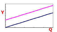
Thus, Y is proportional to Q, if R is held constant. The coefficient a1 is the constant of proportionality. It is also the slope of the line of Y vs. Q with R held constant. If the value of R were changed, the slope of Y vs. Q would still be a1. Thus the plot of Y vs. Q would just be shifted up or down:

In this model a₀ is the intercept, the value of Y when all of the independent variables are set equal to zero. Since a₁ measures how much Y changes as Q is changed, it is a measure of the sensitivity of Y to Q. Similarly, a₂ is a measure of the sensitivity of Y to R. (In mathematical terms, a1 is the derivative of Y with respect to Q.) An important limitation of MLR models is that the sensitivity is constant and does not depend upon any other variables.

The coefficients of the MLR model are determined by fitting the model to some data by a mathematical procedure, similar to what was done with simple linear regression.
In some cases a modeler may want to consider many independent variables, but is not sure which ones are important.

Regression software is able to test which ones contribute significantly to the predictive power of the model, and the modeler can weed out those that don't. For example, see the Retail Store Application. In that case thirteen independent variables were tested, but only two were found to be significant by MLR.

MLR is probably the most widely known and used empirical modeling technique. In spite of the limitation that its sensitivity is constant and independent, this is a very powerful procedure to determine what variables affect an outcome, and to quantitatively predict what that outcome may be. Many real systems can be accurately modeled with it, as long as the model is restricted to a range of conditions in which the assumption of constant and independent sensitivity is valid. This can be checked by a variety of graphical and statistical means (see Draper and Smith).

Multivariate Polynomial Regression (MPR)

However, the assumption of constant and independent sensitivity cannot be made for many other systems. Suppose the sensitivity of Y to Q depends upon R as in the following plot:

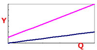
Here one line represents Y vs. Q at one level of R, and the other line is Y vs. Q at a different value of R. An example would be crop production vs. nitrogen at different levels of irrigation. More irrigation allows a plant to take advantage of increased fertilizer levels.

Thus the sensitivity of a crop to nitrogen increases if irrigation is increased. When the sensitivity of an outcome to an independent variable depends upon the level of another independent variable, the two independent variables are said to interact.

If one conducted an experiment in which a number of fields were treated with varying levels of nitrogen fertilizer and irrigation, and the data were fitted by multilinear regression (MLR) model, interaction behavior would be missed and the model would predict the wrong sensitivity. This is a kind of model bias.

An unbiased model can be off due to random factors, but if the data were accurately measured, such as by repeating the measurement and averaging the results, then the prediction would become more accurate.

In a biased model, there will be some error no matter how accurately you make your measurement. If your data shows an interaction effect and your model isn't capable of producing it, then your model will be biased.

Interaction as shown in the figure above can be incorporated into the multilinear regression model by adding an interaction term consisting of the product of the two independent variables, Q·R:

Y = a₀ + a₁·Q + a₂·R + a₃·Q·R

The sensitivity of Y to Q in this model (the derivative of Y with respect to Q) is a₁ + a₃·R. Thus, as expected, the sensitivity depends on the value of R. (Note that the intercept, the value of Y when Q=0, is also a function of R: a₀ + a₂·R.)

Data can have even more complex behaviors. For example, the plot of Y vs. Q could be curvilinear, and the curvature could depend upon R. The nest figure displays this kind of situation.

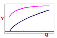
In the above figure, the blue line represents Y vs. Q at one level of R, and the magenta line is Y vs. Q at another value of R. This shows a saturation-type behavior (Y seems to be tending towards a limiting value as Q increases). This is a common behavior, but no linear model is capable of describing it.

Curvature can be included in a model by adding terms with powers other than 1.0. For example, if the list of allowed exponents were {1, 2}, then parabolic shapes could be described. In the example of Y as a function of Q and R, we could try terms consisting of Q², R², Q²R, QR², and Q²R². Altogether, we could wind up with a model with nine terms like this:

Y = a₀ + a₁·Q + a₂·R + a₃·Q·R + a₄·Q² + a₅·R² + a₆·Q²R + a₇·QR² + a₈·Q²R²

If there were three independent variables, we could have as many as 27 terms in the model. But it doesn't end there. To describe even more complex shapes we might need higher exponents. If we included exponent 3, we would need terms such as Q3, Q3R, or Q3R3, and the total number of terms would be 16. If there were three independent variables, there are 64 possible terms.

If there are only one to three independent variables, higher dimensional relationships such as these can be discovered by graphical analysis. However, if there are many independent variables, then there is no direct way to do this, other than by statistical analysis.

You can see that the models start to get too complicated as the number of variables and/or exponents increases. Besides complexity, there are other important problems that can occur. If the number of terms approaches the number of data point used to fit the model, the model may become too good at fitting the data, in the sense that it starts to fit the quirks of the data that do not generalize to new data. If you collected more data that were not used in the fitting, and checked the ability of the model to describe the new data, you would find that it does poorly. This is called overfitting. It can be controlled by limiting the number of terms in the model. A rule of thumb is to have six to ten times as many data points as there are terms in the model. However, this depends upon the amount of noise in the data. If there is little noise, then the number of parameters can more closely approach the number of data points.

A form of overfitting is interpolation. In interpolation, the number of parameters in the model equals the number of data points, and the model goes exactly through each point. There is zero error. For example, as is well known, if you have two points, you could fit a straight line exactly through the points. That gives an equation with two parameters: the slope and intercept. A quadratic equation (second degree polynomial) can exactly fit three points, and a tenth-degree polynomial can exactly fit nine points. This may be desired in some situations, but, especially with high-degree polynomials, even the slightest error produces a behavior called polynomial wiggle, in which the model doesn't behave well in between the data points. Interpolation and polynomial wiggle are prevented by having sufficiently fewer parameters than data points. The difference between the number of data points, n, and the number of parameters, p, is called the degrees of freedom, df = n - p. In interpolation df = 0.

Polynomial wiggle, along with other challenges for polynomial models including nonlinear bias and explosive behavior are described here.

Another potential problem is called chance correlation, in which the data show effects that are actually present due to random variation. If another dataset were collected, the same effect probably wouldn't show up. Another technique that controls both overfitting and chance correlation is called cross-validation, and is described below.

The number of terms can be limited in several ways. One is to limit the number of exponents. Another is to limit the number of multiplicands allowed in each term. For example, if there were five independent variables (Q, R, S, T, and U) we could eliminate terms with more than two of them at a time. Terms such as S²T or QU would be allowed as candidate terms, but RS²T, QRU, or QR²S²TU would not. A maximum of two or three multiplicands seems to work well in many cases.

However, these methods (especially limiting exponents) could limit the ability of the model to describe the complexity in the data. Another way to limit model complexity is to weed out individual terms that don't contribute to the predictive ability of the model. The statistical technique of regression includes methods to determine which terms are significant. Typically, only a few terms may be necessary. For example, the previous nine-term model might be reduced to the following three-term one:

Y = a₁·Q + a₃·Q·R + a₆·Q²R

A model can be reduced in this way by a procedure called stepwise regression. In step-wise regression, terms are sequentially added to and removed from the model using the list of candidate terms (all the possible terms given the user-selected list of exponents and multiplicands) until the model's ability to predict the data cannot be improved either by adding or by removing a single term. With step-wise regression, the number of exponents can be allowed to be much greater than otherwise possible.

Note that MPR does not necessarily produce a unique model. That is, one can sometimes find models containing different terms that produce a similar fit. This can be because of multicollinearity, where different polynomials can produce approximately the same shape. This is most common when the data have significant amounts of noise.

TaylorFit Software

TaylorFit software makes the process of fitting MPR models simple. After you specify the exponents and the number of multiplicands, you then enter the fitting process, which consists of repeated fitting cycles, each consisting of two steps. In the first step, each of the candidate terms is added to the current model one-at-a-time. Each of these augmented models is then tested for goodness-of-fit (by one of several criteria), and sorted to select the best. If the best augmented model is significantly better than the current model (again, by using a statistical test of significance) then the augmented model becomes the current model.

In the second step of the cycle a group of models is tested, each consisting of the current model with a different one of its terms removed. If removal of any one term significantly improves the model, then THAT model becomes the new current model. The entire cycle is then repeated until the model cannot be improved either by adding any term from the list of candidate terms not in the current model, or by removing any of the terms in the current model. The user may then choose to change the fitting parameters, such as by adding more exponents, or the user may be satisfied with the current model and stop.

It is recommended that all fitting be done with a multilinear model first, and then proceed to a multivariate polynomial. In other words, the list of exponents should initially be limited to {1}, and the list of multiplicands limited to {1}. Later each list could be expanded a step at a time, until the user is satisfied.

Note that the exponents do not necessarily have to be positive integers. They may be fractional or even negative. Using the exponent set {1, -1} allows ratios of variables to be tested.

However, if any of the independent variables contain zeros, you cannot use negative exponents. Basically, the user should increase the exponents sequentially until the model cannot be further improved. There is some art to selecting the list of exponents and knowing when to stop adding to the list. This will be gained with experience in fitting MPR models.

The repeated cycles can be done automatically, or the user may select a manual mode. In manual mode the software stops after each step and displays the ten best choices. The user may then select one, and proceed to the next step.

Errors and Goodness-of-Fit Statistics

All measurements contain noise. Thus if we expect data points to fall on a line, we would actually find them scattered somewhat on either side, as shown in the example below:

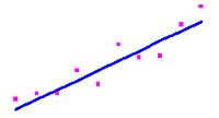
A good model is one that keeps the error small. However, we can't just pick the line that minimizes the total error because it turns out that it's always possible to pick a bad model that gives a total error of zero. This is because you can arrange to have large positive errors cancel out large negative errors.

For reasons we won't go into here, one of the best measures is the sum of the squares of the errors, which we abbreviate as SSE. This is the most basic measure of how good a model is. In fact, the method used to fit the MPR model, called least squares regression, is essentially a mathematical procedure that picks the coefficients that minimize the SSE.

However, SSE alone is not a good measure of goodness-of-fit of the model. This is because we can always decrease SSE by adding more terms to the model, even though we would be overfitting the data. In fact, if there are as many terms in a polynomial model as there are data points, the model can go right through every point, giving SSE equal to zero. This situation is called interpolation, and is not desired unless we are dealing with negligible measurement error.

Instead, there are a number of other goodness-of-fit statistics, all of which are based on the SSE. For example, we could divide SSE by the degrees of freedom. This is called the mean square error, or MSE. That is,

MSE = SSE/df

If we add too many terms to the model, the MSE can increase even if SSE decreases. The MSE is a measure of how much the data points are spread out from the model line (i.e. it is an estimate of the variance of the error).

Another, and probably the best-known, goodness-of-fit statistic is the coefficient of determination, better known as the R² value. The R² is based on the SSE such that it has a value of 1.0 when SSE equals zero (the best situation), and it goes to 0.0 when SSE is a maximum. However, like SSE, it can always be improved by adding terms, which does not necessarily mean we have a better model.

Another important goodness-of-fit statistic is the F-statistic. The F is computed using the MSE, and can be used in turn to compute a significance level. The significance level gives the probability that the model fit the data by just by chance. Typically, modelers prefer to see a significance level of 5% or less. The F-statistic that gives a 5% significance level depends upon the number of terms and the number of data points. For example, if there are 30 data points and five terms in the model, the F-statistic should be 2.6 or greater for a significance level of 5% or less.

This means that if the F-statistic in this case is greater than 2.6, then there is less than a 5% chance that this correlation occurred purely by chance.

Other statistics for overall goodness-of-fit are the Akaike information criterion (AIC) and the Bayesian information criterion (BIC), which are computed by Taylorfit.

Another important statistic should be discussed here. The t-statistic, as it is used in the TaylorFit software, is similar to the F-statistic, but instead of being used to check the overall goodness-of-fit of the whole model, it is used to check individual terms in the model. With 30 data points and five terms in the model (25 degrees of freedom), the critical value of the t-statistic for a 5% or lower significance level (or probability that the term fits by chance) is 2.06.

That is, as long as the t-statistic for a term is greater than 2.06, we should keep it in the model. To be even more conservative, one could use a 0.5% significance level. In this case the critical value of the t-statistic for 25 degrees of freedom is 3.08.

In the stepwise regression procedure described above, one of the above criteria is selected. Then terms are added to or removed from the model if they improve the overall goodness-of-fit (in terms of MSE, F-statistic, AIC, or BIC), or if the term has a value of the t-statistic greater than the critical value for adding, or less than the critical value for removing the term. Using MSE tends to result in more terms being added to the models. The F-statistic is the most conservative, resulting in the fewest terms in the final model.

Example of MPR for Correlation

See the Retail Store Example to see how MPR modeling is used for multivariate nonlinear regression analysis.

Cross-validation

Cross-validation is a technique for greatly reducing problems such as overfitting and chance correlation. TaylorFit has a built-in capability to do cross-validation.

Cross-validation is the preferred technique. It should always be used when possible. The problem is that it requires more data, which are not always available.

In cross-validation, the data are divided into two sets. The first is called the fit dataset, the second is the test dataset. The fit dataset is used for the regression directly. That is, the coefficients of the model are computed by regressing the model to the fit dataset. However, the decision about whether a model is improved over other models with different terms is made by looking at how well the model predicts the data in the test dataset. We make this judgment by computing one of the goodness-of-fit statistics with the test set. This could be any of the ones computed by TaylorFit: R2, MSE, F-statistic, AIC, or BIC.

For example, in the retail dataset described above, we could have used half the data for fitting, and half for testing. The first half is used to compute the coefficients of a candidate model by using the regression calculation. The candidate model is then used to predict the gross margin using the data in the second half of the dataset, and the MSE is computed. This is done using all the candidate models. The candidate model that produces the smallest MSE is then selected as the new current model.

An important consideration in dividing your data into fit and test sets is that they should both have similar behavior. For example, they should cover similar ranges of each variable, or a plot of the dependent variable vs. each independent variable should cover a similar region of the graph. This can be checked by plotting the data and by examining histograms of each variable in each dataset. If one of the two datasets contains an outlier that is not in the other dataset, the fit will be poor.

Time-Series

Often, the data are measurements taken at regular intervals - once per minute, once per day, etc. Examples include stock market indices or daily measurements of flow in a river. Such data are called time-series data. In making predictions about time series, it helps to know not only what is influencing the output currently, but also what its previous value was. For example, the Dow Jones Industrial Average (DJIA) today will depend not only on the latest bond rates, but also on what the DJIA was yesterday. This dependence upon previous values of itself is called autocorrelation.

In modeling time-series, we need to treat previous values of the dependent variable, as well as previous values of the independent variables, as additional independent variables. Previous values of a variable are called lagged variables. They can be lagged by one or more time steps. For example, a model to predict the flow in a river may depend the previous two days measurements. We could say that lag 1 and lag 2 are used as independent variables to predict the current value (lag 0).

If we had many years worth of data for the river, we might make use of the fact that the flow has some dependence on the season. Therefore, to make a prediction we would want to use not only the flow from yesterday and the day before, but from a year ago today. Thus the lags we would use would be {1, 2, 365}. This is called a seasonal effect. This doesn't only imply calendar seasons. It could also be used to model weekly effects on a daily variable (using lag 7) or daily effects on an hourly variable (using lag 24), etc.

TaylorFit software has the capability to include lagged variables. The user specifies a list of the lags to be considered (for example, {1, 2, 365}, as described above).

In some cases, there might only be a single variable which serves as both dependent and independent variables.

For example, if we had a time-series of river flow data, we could still model it, say by predicting today's flow using yesterday's and the day before. This situation is called a univariate time-series. If, on the other hand, there was one or more other variables that could be used to predict a variable, as well as lagged variables, we would have a multivariate time-series. To continue with the river flow example, there might be data on rainfall as well as river flow. We could then use lagged values of rain and river flow to predict current river flow.

Another example of a multivariate time-series is the Lydia Pinkham data. This is a well-known dataset containing annual sales income and advertising budget for a company. Using these data, one could predict sales using the previous year's sales and previous year's advertising budget. When multivariate time-series are modeled using MPR, the resulting type of model can be called a Polynomial AutoRegressive eXogenous variables model, or PARX model.

Example PARX Model

See the Lydia-Pinkham Example to see how MPR modeling is used for multivariate nonlinear time-series analysis.

Vector PARX Models

A final level of complexity occurs if there are several variables that change together, all of them depending upon each other. An example is that of predators and prey populations. The number of predators in an ecosystem depends upon the number of prey available for food, and the number of prey is affected by the number of predators that limit their abundance. In this case, we would need to develop two models. In one the prey is the dependent variable, and lagged values of both predator and prey could be used as independent variables. In the other model the predator is the dependent variables, and we would use the same independent variables as the prey model. Both models would have to be run together to make predictions, since they are coupled together. Models of this sort are called vector autoregressive (VAR) models. Of course, many types of models could be used to describe each population, but if the PARX model is used, we can call this type of model a vector PARX (VPARX) model.

Example VPARX Model

For a particularly challenging example of a vector autoregressive model, see the section on modeling the Lorenz Equations. These are a set of three equations that exhibit a behavior called chaos, which is a highly nonlinear situation.

Discriminant analysis